Equalization - it stands for equalization

Believe it or not, there are many electronic processing techniques that are used in the composition of today’s top songs. Some of these processing techniques are standard and are used to create the high-fidelity recordings we’re used to listening to. Other techniques are used in a more artistic way and employed to create a specific effect. We’re going to look at some of the most common electronic processing techniques and effects, where they are used, and a little bit of the history behind them. As we do, keep in mind that I will be mostly covering these processes as they relate to digital production. Most if not all of these techniques were first invented using analog technologies, and learning about analog signal flows can be incredibly enlightening to how the technology actually works. Ultimately, though, that is far beyond the scope of our class.

Anyways, let’s dive in!

EQ and Frequency Manipulation

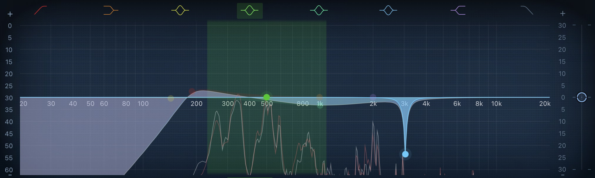
Let’s start with equalization, a form of frequency manipulation that is found in almost all kinds of music. Equalization, or EQ, can take place across all points of a song’s production, including in the shaping of electronic instruments, the composition process itself, and in post-production to clean up recordings. EQ is used to filter out set frequencies of an audio signal with several types of filters that help describe what frequencies are being attenuated (brought down) or boosted in volume. This includes low-shelf & high-shelf, low-cut & high-cut, low-pass & high-pass, bandpass, and notch. I’ve provided a snapshot of what these filters look like using Apple’s EQ found in Logic. Keep in mind that lower frequencies are those lower in pitch and are situated on the left of the spectrum. Higher frequencies are those higher in pitch and are positioned at the right of the spectrum. The verticle axis displays relative volume across the whole spectrum.

A low-shelf filter attenuates or boosts lower frequencies across a wide range. Low-shelf filters may be used to provide extra volume to the fundamental frequencies of basslines, low drones, and percussion without altering their higher harmonics. Meanwhile, a high-shelf does the same process just for higher frequencies.

A low-cut filter, as the name implies, completely cuts out lower frequencies past a certain defined frequency. This can be used to remove unwanted noise found in the recording process, such as cable interference. This filter may also be referred to as a high-pass filter since it is allowing all of the higher frequencies to pass through.

A high-cut filter would then completely cut out higher frequencies past a specific, defined frequency and would be synonymous with the low-pass filter. The high-cut filter can be most useful in cutting out unwanted noise that is higher in pitch, such as room noise and unwanted sounds from far away.

These filters have two pretty distinct effects when taken to their extremes. A low-cut/high-pass filter creates a sort of low fidelity sound when filtered. Meanwhile, a high-cut/low-pass filter muffles all of the high frequencies, making it sound as if the audio is in another room or underwater.

A band-pass filter is similar to the other pass filters in that it allows some frequencies to pass through while blocking others. Band-pass filters instead have a range, or band, of frequencies that are allowed to pass through with cuts on both ends of the range to block those frequencies.

A notch filter is kind of the opposite of pass filters. Instead of allowing a wide range of frequencies to pass through, a notch filter can be used to attenuate or completely cut out a very narrow range of frequencies. For example, there may be a very specific ringing or room noise you want to remove from your audio track. By analyzing the waveforms and finding the frequency of that noise, you can use a notch filter to remove without affecting the rest of the track. While a notch filter could be technically used to boost these frequencies, I’m not sure of any practical use in that besides specific and niche composition goals.

There are many other shapes you can find in an EQ graph. By combining these filters and changing other factors associated with them, you can begin to craft specific timbral sounds that are used in electronic instruments or simply used on a raw audio signal. Additionally, these factors can be programmed to change overtime over the course of a track. This is called automation and is a function found in every digital audio workstation, and can be employed with every kind of electronic processing. A common automation technique for EQ is the changing of the cut-off frequency for the cut-off filters. This creates a sweeping sound that gradually takes out high or low frequencies - depending on whether it’s a high-cut sweep or a low-cut sweep.

Fading and Cross-Fading

Fading refers to the process of taking the volume of an audio file in or out from absolute silence. This is most common at the begging and end of full songs, where the audio gradually comes in from silence over an extended period of time or fades into absolute silence at the end. Additionally, fades can be used on specific tracks at a time within a multi-track mix. This allows us to bring in or take out instruments seamlessly from the mix.

Cross-fading refers to two or more tracks fading in and out of one another simultaneously. Modern DAWs can handle this automatically and allow tracks to seamlessly overlap each other, or it can be done manually across multiple tracks. This technique is most common in pop tunes where multiple instrument tracks are used at different points in the song. Quick cross-fades allow for the seamless transition between instruments/sections without an abrupt and out-of-place change in timbre.

Fades can also be used technically when working with many raw audio files across multiple tracks, especially if they are cut up from longer waveforms. When cutting an audio file in the middle of a waveform, artifacts known as “clicks” occur when the waveform is abruptly cut off. To mask these “clicks,” tiny fades can be used at the beginning and end of the cut audio file. The fade is so small that a change in volume is imperceivable, but the “click” will have been completely faded out. This is most often employed in electronic pop, especially EDM music that may sample other songs. Since these samples are cut out of the context of the original song, a “click” is inevitable and so these minuscule fades are used in between each sample. Listen to the last audio example here. The first playing will be an audio file that does not have a fade-out. If you listen carefully you should hear a click. The second playthrough has a fade-out.

Spatialization

Spatialization is the placement or movement of sounds across multiple channels. In most cases, the number of channels musicians work with is 2, left and right, which is called stereo. Many electronic music composers work with up to 8 channel set-ups, while movie theatres can have up to 12 channels. In most cases, the number of channels directly correlates with the number of speakers in a room. Think of your car stereo, which (probably) has only 2 speakers, while a full IMAX movie theatre would have 12. You may see the expression of these channels like this: 2.1, 4.1, 8.1, 12.1. The first number is the number of channels in the sound system, while the second number is the number of sub-woofers - an extra speaker specially designed for low frequencies.

Modern pop, or at least audio engineers who produce it, have the spatialization of stereo listening down to a science. They know just how far left or right to pan the guitar tracks while balancing the percussion across both channels while feeding the vocals into both channels. While not always evident when listening in our cars or from our laptops speakers, these choices of spatialization are very noticeable when listening through headphones or home theatre systems. In fact, if you regularly listen to music while driving, you may be surprised by new sounds coming from the right channel when listening on headphones since that speaker may be blocked by a seat or a person normally.

While this is a great start to spatialization, it only scratches the surface. Any piece of music can change spatialization seemingly in real-time. This is either done through automation like EQ, but also manually through the panning of tracks - this is especially evident in pieces with 4 or more channels. Listen to the example here - ideally on a computer with 2 speakers - and notice how the sound changes its place as I pan back and forth. This is an incredibly simple example with just one track, but can just as easily be done across multiple tracks with multiple instruments to create some pretty awesome sound experiences!

Basic Tape Techniques

In the first couple of modules, we talked about the analog technique of breaking and skipping as it related to early hip-hop. This concept was foundational in the technique of sampling, where a specific portion or track is taken and recontextualized into a different song. Before the use of vinyl records, though, magnetic tape was the premier technology for music recording, thus music processing. Common commercial uses for music imprinted on tape were cassette tapes or VHS tapes for film. The four basic tape techniques used in music production are cutting, splicing, reversing, and speed.

Cutting is the process of taking a single audio file in a track and cutting it into two portions. Cutting can and often does happen multiple times across a single audio file. The most common use for cutting audio is to remove an unwanted portion of music/sound or to prepare a sample out of the cut material. The term itself, as you could imagine, was derived from the physical cutting of magnetic tape strips.

Splicing is the opposite of cutting, where you combine the ends of two audio files into a single file. In my experience of working with digital audio, splicing is not nearly as common as cutting. This is because splicing together two waveforms can cause those unwanted “click” sounds. Since we have the capacity to work with a virtually unlimited amount of tracks, musicians and engineers often opt to use multiple tracks with fades or crossfades to simulate the splicing of audio. Again, the term comes from the physical action of combining two ends of magnetic tape strip together to create a seamless line of tape.

Reversing is the process of taking an audio file and - well - reversing it. In digital media, this process is handled automatically through the analysis of a waveform which is then reconstructed in reverse. On analog tape, this would be accomplished by recording a sound on tape and then rolling it backwards to re-record on a new tape (the master track intended for listening), or cut and physically turning it around.

Finally, tape speed refers to changing the speed at which the audio is heard. This can be slower or faster than the original sound. There’s also a funny quirk that happens when altering tape speed. The faster a tape is sped up, the higher it will be in pitch. The slower a tape is heard, the lower in pitch it will be. This can easily be accomplished with digital audio as well, and there are even special tools that can be used to change the speed of an audio file without changing its pitch. In Logic, this tool is called “flex-time.”

When used in combination, these four incredibly simple techniques can create a virtually infinite playground of processing in recording, performance, and composition. The concepts loosely translate to vinyl records as well as recognized with breaking and skipping earlier. Today, the analog techniques used with tape or vinyl records can all be done digitally. In fact, most modern processing techniques found in DAWs can be traced back through these analog technologies including delays and degradation - let’s look at these next!

The spectrum of Delays

With digital media, delay refers to the repetition of a signal at a set time after its original pass. The simplest way to conceptualize this is with echos. When you talk or make a noise in an empty room, canyon, or another space with hard surfaces, the sound waves from the sound will bounce off these surfaces and come back to you. In the supposed canyon, the echo sound will have a perceivable lapse in time, full seconds from when you first made the sound. The reverberation made in a small, empty room will barely have a perceivable lapse in time, creating a boomy effect to the sound. These effects are just two of the several delays that make up the spectrum, and we can analyze them both temporally and in effect.

As alluded to before, reverb (short for reverberation) is the shortest kind of delay hardly sounds like a delay at all. Reverb delays a signal multiple times within a few millisecond windows causes the initial signal and the subsequently repeated sounds to all blur together. The effect is most often used to artificially simulate music being played in a live space, and once can tweak the variables of reverb equipment to create different room sounds.

Flanger and chorus are two kinds of delays that use the foundation of the concept of reverb to create two unique effects. A flanger takes two identical audio signals and delays one of them by a few milliseconds at a time while also changing the time scale of each delay - usually 10-40 milliseconds. This causes the two audio signals or more to come in and out of phase with each other creating a ‘swooshing’ sound that is similar to an EQ sweep. The signals being “in-phase” means they are identical to each other, while “out-of-phase” is when the delay pushes one of the signals to not be directly lined up with the unaltered ones. This happens in a cycle with the signals syncing and desyncing from another, which creates the back and forth ‘swooshing’ sound. A chorus also takes two or more signals at a time. Instead of modulating (changing) in time, a chorus delay modulates the pitch of the delayed signals. This creates a sort of imperfect tuning sound coming from multiple voices - apparently as heard in singing choirs.

A little longer than reverb, flanger, and chorus delays is the slapback echo. The slapback echo is incredibly prominent in rock music and can be found in many kinds of guitar effects pedals. The slapback echo usually only delays a signal once at about 100-200 milliseconds with no other changes to the signal. This creates a discernable echo in the signal that often blends into the original signal.

Finally, we have generic delays and echos. As far as my work with electronics has brought me, I use these terms interchangeably. However, somebody may technically assume that an echo is a delay that only decreases in volume across every repetition, much like a natural echo. Meanwhile, a delay takes the temporal length of an echo while also modifying other factors, including increasing volume, changing spatialization, or changing timbre. At this point, the terms are used to describe delayed signals that are longer than 200 milliseconds or so.

As with every single processing technique so far, all of these delays can be combined with other processing techniques, including specialization, pitch, and amplitude. Given the right tools, one can even change the processing of each subsequent, individual signal within a delay, generally referred to as multi-tap delays.

Distortion and Degradation

Distortion, as the name suggests, is the intentional or unintentional destruction of an audio signal. In digital audio, distortion is created by raising the amplitude of a signal past a set cut-off point. Hitting the upper and lower limits of amplitude for a system creates an artifact known as “clipping.” When done intentionally and for a prolonged time, we can create audio effects that most of us are familiar with. The timbre of the distorted audio signal is controlled by multiple factors including the initial signal, the amplitude cut-off, and how the clipped sound is interpolated (known as soft and hard clipping)

Degredation, also known as decimation and downsampling, is another type of destructed signal. Instead of destroying via amplitude, degraded signals are degraded by reducing a signal’s sample size. Remember that digital audio signals are representations of analog, mechanical waveforms that are recorded in real-time. In order to be converted into digital audio, an analog signal must be sampled at a certain rate in order to capture the signal and represent it faithfully. You can think of a sample as a single snapshot picture of a waveform. Multiple snapshots, or samples, are taken every second in the audio. When all of these samples are put together, they create a faithful digital recreation of the sound captured - just like multiple pictures taken in quick succession and played resemble a movie.

Knowing how samples work, we can intentionally down-size the sample rate of audio in the process known as degradation. The lower the sample size of a waveform, the less information we have to faithfully recreate the original audio. With so few samples, the digital audio will represent the audio with what information it has. The lower the sample size, the less information captured, the more the signal is degredated. Listen to the example here to hear what that sounds like.

Auto-Tune

Let’s wrap up this module with a look into a well-known and often criticized processing technique: auto-tune. Auto-tune is a specific piece of equipment developed in the late 1990s but is now a generic term that stands in for any process used to correct inaccuracies in music performance. By sampling and analyzing the pitch of a piece of audio, the frequencies can be fudged in any direction to subtly correct issues with intonation and tuning. This is essentially a form of pitch-shifting, and while useful can dull the richness of a raw audio signal. Aside from this technical drawback, auto-tune has historically been criticized in all circles of music as being a crutch used to aid poor performance. However, this leaves us with such a narrow-minded picture of the technology of auto-tune, as ultimately prevents us from seeing it as what it actually is: an audio processing technique!

From my experience, Cher and T-pain were some of the first commercial artists to begin pushing the boundaries of what can be done with auto-tune in the late 90s to early 2000s. By widening the corrective area of analysis and moving between extreme pitch registers, the software creates unique sounding artifacts that redefined auto-tune and modern vocal processing aesthetics.

As technology develops, so do the uses and experiments with vocal processing. Melodyne is another pitch and time-shifting software similar to Auto-tune. Despite being a professional-level software plug-in used in the industry, it has been making the rounds on shorts and Tik Tok as folks pitch/time-shift popular songs into another dimension. In the next module, we will also be looking at a piece that also utilizes these techniques in some really inventive ways too!